Multiple Linear Regression

Multiple Linear Regression is an extension of linear regression where we predict the value of a dependent variable (Y) based on multiple independent variables (X₁, X₂, X₃, ....). It models the relationship between the dependent variable and multiple predictors using the equation:

Y = b₀ + b₁X₁ + b₂X₂ + ... + bₙXₙ + ϵ

Where:

• Y: Dependent variable
• X₁, X₂, ..., Xₙ: Independent variables
• b₀: Intercept (value of Y when all Xᵢ = 0)
• b₁, b₂, ..., bₙ: Coefficients representing the effect of each Xᵢ on Y
• ϵ: Error term (difference between actual and predicted Y)

---

Example: Predicting House Prices

Suppose we want to predict house prices based on three features: size of the house (X₁), number of bedrooms (X₂), and distance to the city center (X₃).

Data

House Size (sq ft) ((X₁))	Bedrooms ((X₂))	Distance to City (miles) ((X₃))	Price ((Y))
1500	3	5	400,000
2000	4	3	500,000
2500	4	2	600,000
3000	5	1	700,000

Regression Equation

Using multiple linear regression, we fit the following equation:

Y = b₀ + b₁·X₁ + b₂·X₂ + b₃·X₃

Assuming the computed coefficients are:

• b₀ = 50,000: Intercept (the value of Y when all Xᵢ = 0)
• b₁ = 100: Coefficient for X₁ (per square foot)
• b₂ = 10,000: Coefficient for X₂ (per bedroom)
• b₃ = -20,000: Coefficient for X₃ (per mile from the city)

The equation becomes:

Y = 50,000 + 100·X₁ + 10,000·X₂ - 20,000·X₃

Prediction

For a house of size 2200 sq ft, 3 bedrooms, and 4 miles from the city:

Y = 50,000 + 100(2200) + 10,000(3) - 20,000(4)

Y = 50,000 + 220,000 + 30,000 - 80,000 = 220,000

The predicted price is $220,000.

---

Advantages of Multiple Linear Regression

1. Captures Relationships: It identifies the influence of multiple factors on a dependent variable.
2. Predictive Power: It enhances prediction accuracy by incorporating multiple variables.
3. Quantifies Impact: Provides insight into the effect of each independent variable.

---

Limitations

1. Multicollinearity: When predictors are highly correlated, it can distort coefficient estimates.
2. Overfitting: Too many predictors relative to the data size can reduce model generalizability.
3. Linearity Assumption: Assumes a linear relationship between predictors and the outcome.

---

Multiple linear regression is a cornerstone of statistical modeling and machine learning, widely used in fields like economics, healthcare, and marketing for predictive analysis.

code to predict house prices

# Importing necessary libraries
import numpy as np
import pandas as pd
import matplotlib.pyplot as plt
from sklearn.linear_model import LinearRegression

# Creating the dataset
data = {
    "House Size (sq ft)": [1500, 2000, 2500, 3000],
    "Bedrooms": [3, 4, 4, 5],
    "Distance to City (miles)": [5, 3, 2, 1],
    "Price": [400000, 500000, 600000, 700000]
}

# Convert to DataFrame
df = pd.DataFrame(data)

# Features (X) and Target (Y)
X = df[["House Size (sq ft)", "Bedrooms", "Distance to City (miles)"]]
Y = df["Price"]

# Linear regression model
model = LinearRegression()
model.fit(X, Y)

# Coefficients and Intercept
b0 = model.intercept_
coefficients = model.coef_

# Predict prices based on the model
df["Predicted Price"] = model.predict(X)

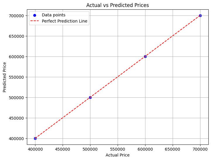
# Plot actual vs predicted prices
plt.figure(figsize=(8, 6))
plt.scatter(df["Price"], df["Predicted Price"], color='blue', label='Data points')
plt.plot(df["Price"], df["Price"], color='red', linestyle='--', label='Perfect Prediction Line')
plt.title("Actual vs Predicted Prices")
plt.xlabel("Actual Price")
plt.ylabel("Predicted Price")
plt.legend()
plt.grid(True)
plt.show()

# Display coefficients and intercept
b0, coefficients